Case Study : The Pygmalion Effect, in SAS - Two Way ANOVA

Case Study: The Pygmalion Effect
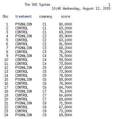
There are 10 army companies each with 3 platoons. One platoon is randomly picked for Pygmalion treatment and the other platoon are control groups. The platoon leader is told his platoon has scored highly on tests that indicate they are superior. After basic training, platoons are given a weapons test. 

The response variable is an average score on basic weapons test per platoon.
There are two factors; company 10 levels(Company 1 ~ 10) and treatment 2 levels (Pygmalion, control) Therefore, there are 19 (=9+1+(9*1)) explanatory variables.

The data is following below.

Reference : Ramsey and Schafer (1997) The Statistical Sleuth, Duxbury Press, p. 365. The Pygmalion effect.


1. Two Way ANOVA with Interaction (Interaction Model & Hypothesis)  
The model with interaction :
$Y_{i}=\beta_{0}+ \beta_{1}I_{pyg,i}+ \beta_{2}I_{comp1,i}+...+\beta_{10}I_{comp9,i}$
                                        $+\beta_{11}I_{pyg,i}\cdot I_{comp1,i}+...+\beta_{19}I_{pyg,i}\cdot I_{comp9,i}+e_{i}$

$H_{0}:\beta_{11}=\beta_{12}=...=\beta_{19}=0$ (all possible interactions)
$H_{1}$ : at least $\beta_{1i}$ is not equal to 0

1.1 SAS Code and Result
 
We can create the Two-Way ANOVA by using proc glm. There are two factors; company and treatment. And we are also interested in interaction terms so that out model should be score=company | treatment, which | creates interactions. The another way to create interaction term is score=company treatment company*treatment.  
 

After running the SAS code above, the overall ANOVA results are following below.

In the interaction (company*treatment), the F value is 0.67 with high P-value (0.7221).
As we get a high P-value, we fail to reject the null hypothesis which means all possible interaction terms can be considered to 0. Therefore, our next model is an additive model which excludes the interaction terms.


2. Two Way ANOVA w/o Interaction. (Additive Model & Hypothesis)
The model w/o interaction:
$Y_{i}=\beta_{0}+ \beta_{1}I_{pyg,i}+ \beta_{2}I_{comp1,i}+...+\beta_{10}I_{comp9,i}$

2.1 The First Question - SAS Result and Conclusion 
Our first question is there is a difference in mean score between Pygmalion and the control groups!!
$H_{0}:\beta_{1}=0$ 
$H_{1} : \beta_{1}$ is not equal to 0

As our interest is to find a difference between Pygmalion and the control groups, so we need to look at the treatment source. As we have a small P-value (0.0119), so we reject the null hypothesis which means there is a evidence of a difference in mean score between them.
Note that F value is distributed by F(# beta being tested, # degrees of freedom of SSE) = F(1,18)

However, in the diagnostics for score matrix, we can see a decreasing variance estimate pattern. Even though we have a small P-value, the evidence of our conclusion is week.

2.2 The Second Question - SAS Result and Conclusion
Our second question is there are differences in companies!!
$H_{0}:\beta_{2}=\beta_{3}=...=\beta_{10}=0$ 
$H_{1}$ : at least one $\beta_{2}...\beta_{10}$ is not equal to 0
 

As our interest is to find a difference among 10 companies, so we need to look at the company source. As we have a high P-value (0.1484), we fail to reject the null hypothesis which means there is no evidence of difference among companies. 
Note that F(9,18) = F(# beta's being tested which are beta 2~10, # d/f of SSE)

Combining two question conclusion, our final model will be $Y_{i}=\beta_{0}+\beta_{1}I_{pyg,i}$


3. Model Checking
In the diagnostic panel, we can see whether our assumptions are satisfied or not.
There is no outliers, and normality looks ok. However, we have a concern of decreasing variance. Another assumption is independent observation which we assume that platoons were picked at random and were not interacting. 

Two-Way ANOVA

[1] Two Way Classification or Two-Way Analysis of Variance
This is another special case of the GLM (General Linear Model). In the GLM, the response variable is continuous and the explanatory variable is categorical or continuous. For the GLM information, click here! :D So, the Two-Way ANOVA has two factors, each with at least two levels. The main question is weather the treatment variable have an effect or not.   

What is the factor? A factor is a categorical predictor variable consisting of different class levels like various types of treatments. For example, if you want to predict the grade of the course you are taking, then there are several factors such that the number of hours you are studying, the number of assignments or a female/male student etc. 

[2] Assumptions
The samples must be independent, and selected by randomization condition.
The equal variance assumption and normal error assumption should be satisfied.

[3] Model and the Expected Values Example  
Consider the model for a two-way analysis of variance with two levels of each factor (a 2x2) classification. $Y_{i}=\beta_{0}+\beta_{1}I_{factor 1,i}+ \beta_{2}I_{factor 2,i}+\beta_{3}I_{factor 1,i}I_{factor 2,i}+e_{i}$ where $I_{factor 1,i}$ if the ith observation is in the first group of factor 1 and is 0 otherwise.

**The expected values of $Y_{i}$ for each of the 4 groups means are following.
1) i : 1st level of the factor 1, and 1st level of factor 2 : $E[Y_{i}]=\beta_{0}+\beta_{1}+\beta_{2}+\beta_{3}$
2) i : 1st level of the factor 1 and 2nd level of the factor 2: $E[Y_{i}]=\beta_{0}+\beta_{1}$
3) i: 2nd level of the factor 1 and 1st level of the factor 2: $E[Y_{i}]=\beta_{0}+\beta_{2}$
4) i : 2nd level of the factor 1 and 2nd level of the factor 2: $E[Y_{i}]=\beta_{0}$  

[4] The Full Model & The Reduced Model and Test Statistics 
The full model is a model with all explanatory variables, whereas the reduced model (or additive model) is a model without variables whose coefficient you are testing.

The test statistics is following below.
$F_{obs}= \frac{(SStrt_{full}-SStrt_{reduced}) / \#of\beta's \ being \ tested }{MSE_{full}}$

[Multiple Comparisons] The Bonferroni Method

 

If we need multiple tests for comparing means with a single data set, there are many pairwise comparisons. For example, when comparing three means(A, B, and C), there are 3 pairwise comparisons, T1=(A,B), T2=(B,C) and T3=(C,A). If there are G groups means, there will be $k=\binom{G}{2}= \frac{G \cdot (G-1)}{2}$ pairwise tests which are T1,...,Tk. 

 

So based on the Bonferroni inequality, $P(A\cup B)\leq P(A)+P(B)$,

P(T1 incurs Type I error) + ... + P(Tk incurs Type I error) = $P(\cup_{i=1}^k A_{i})\leq \sum_{i=1}^k P(A_{i})$

 

For example, let $\alpha$ =P(Type I error)=0.05 and G = # of means = 7, then k=(7*6)/2=21,

then P(at least 1 Type I error) = $1-(1-0.05)^{21}=0.6594$, which means there is an increased chance of making at least one Type I error rate.

P(at least 1 Type I error among independent k tests) = 1 - P(No Type I error among k tests).

 

In order to control to have less than $\alpha$, each of k pairwise tests is done at level $\frac{\alpha}{k}$!! In this example, our adjusted error rate will be 0.05/21=0.0024!! So the probability of Type I error rate in each test should be 0.0024 so that the probability of Type I error rate among 21 pairwise test will be similar to 0.05.
P(at least I type I error) = $1-(1-0.0024)^{21}=0.0492 \approx 0.05$
  

So this Bonferroni method is conservative as we are asking greater evidence which means overall Type I error rate is much less than $\alpha$.

 

The General Linear Model (GLM)

[1] What's the General Linear Model (GLM)?

In GLM, there is a continuous response variable, and one or more categorical/continuous explanatory variables. The response Y is linear in the beta's. In SAS, we use proc glm or proc mixed statement. In R we use lm().  For more information, please refer to the reference below.

Reference: http://support.minitab.com/en-us/minitab/17/topic-library/modeling-statistics/anova/basics/what-is-a-general-linear-model/ 

One way ANOVA is a special case of a general linear model. Of course ANOVA, ANCOVA, linear regression, mixed model also are the GLM. In GLM, we can predict beta by using the least squared or the best linear unbiased prediction. Don't confuse the difference between General Linear Model and Generalized Linear Model later. Let's find out what the hypothesis and assumptions of GLM and what the one-way ANOVA is.

[2] GLM: Hypothesis and Assumptions

The null hypothesis is $\beta_{1}=\beta_{2}=...=\beta_{p}=0$

The GLM assumptions should be the errors are normally distributed with mean 0 and a constant variance, and they are uncorrelated.

 

We can predict the beta with the least squares estimates.

$\widehat{\beta}=(X^TX)^{-1}X^TY$

- The columns of X should be linearly independent, and $X^TX$ should be invertible.  

[3] One Way ANOVA : Assumptions, Table

In the One way ANOVA, the reponse variable is continuous, there is one categorical factor with at least 2 levels. The group variances are equal or at least fairly similar, and the errors are normality distributed. We are not assuming no outliers, also balanced groups are not required. The one way ANOVA table is following.

The P-value is come from high observed F statistics, and this statistics is come from the ratio of variances of two groups. Therefore, the main idea is if the between groups SS is larger than within the groups SS, there is evidence that means are different.

Case Study: The Spock Conspiracy Trial, in SAS (by using proc glm)

Case Study: The Spock Conspiracy Trial in SAS
The main question is there is evidence that women underrepresented on Spock judges venire when compared to other judges?

1. SAS Code
Please refer to the previous post how to read the data file by using infile code, and sort into two groups; 'SPOCKS' and 'OTHER' by using if statement. This SAS code demonstrates how to use proc glm for comparing two groups. The class statement in proc glm makes dummy variables. In order to print the estimates of the beta's, then we need to put the solution statement.

2. SAS Code - Output List

If you run the SAS code above, you can see the result list below. From the class statement, we can see there are two levels, Poscks and Other. And we need to focus on Type III model ANOVA and Solution.   

 

3-(1). SAS Result -  Class Levels

As you can see the result below, there are two levels created, Other and Spocks.

3-(2). SAS Result -  Least Squares Means

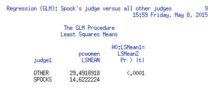
In this SAS output, we can see the least squares means for each level. Our hypothesis is that the LSMeans of the level Spock is equal to the LSMeans of the level Other.

3-(3). SAS Result - glm solution   

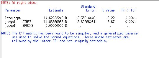
From the solution statement, we can get the estimates of the each beta's. And each parameter has small p-values (less than 0.0001), so parameters are significant.
The equation will be pcwomen = 14.622 + 14.870*Other

3-(4). SAS Result - Type III model ANOVA    
F-value will be given in the Type III model ANOVA output. From the previous post regarding the two sample t-test in SAS, the pooled t-value was 5.67. Note that the squared pooled t-value is equal to the observed F value, which is 5.67*5.67=32.15.

4. Overall conclusion    
In order to compare the means of the two groups, we can use two sample t-test, SLR with 1 dummy variable or one-way ANOVA with two groups by using different statements. Of course each method has the same conclusion!!

Case Study: SLR with 1 dummy variable in R

 

Case Study: The Spock Conspiracy Trial in R
The main question is there is evidence that women underrepresented on Spock judges venire when compared to other judges?

 

1. Prepare Data

If you don't have the data set, just follow procedure below; install a package and load the package. Our case study data set is called "case0502".

 

2. Make a Boxplot
Our goal is to compare the mean values between Spock's and other judges (1~6). First of all, we can make a bloxplot displaying the 5 statistics: minimum, first quartile, median, third quartile, and maximum.  

 

3. Conduct the SLR 

First, we divide into two groups: Spocks' and others by using ifelse function as we want to compare means of two groups. And then conduct the simple linear regression by using lm function. The response variable is the "percent" and the explanatory variable is a "twogroup" which is a dummy variable.  

 

4. Conclusion  

If we use anova( ), then we can see the one-way ANOVA table above. The main idea is that between groups SS (twogroups Sum sq=1600.6) is larger than withing groups SS (residuals sum sq=49.79), there is evidence that means are different. Therefore, as we have a small p-value (1.03e-06), there is strong evidence in mean difference between two groups.  
Remark) We will get the same conclusion if we conduct the SLR. More information, Click! 

 

- Reference: http://www.inside-r.org/node/159733