Case Study : 2X2 Contingency Table in SAS

Case Study : Framingham Heart study 

In 1948, in Massachusetts, 5209 healthy men and women, aged 30-60 were recruited and followed to examine risk factors for cardiovascular disease(CVD). After 10 years, checked whether they developed CVD or not. So main question is high cholesterol is associated with increase risk of CVD. 

 
Reference: https://www.framinghamheartstudy.org/, https://en.wikipedia.org/wiki/Framingham_Heart_Study  
 
 
[1] Data Assumption and SAS Code for reading the data. 
The number of total sample (n) is 1329 (men). The cholesterol was measured in 1948, and after ten years, checked whether cardiovascular disease (CVD) was found or not. Therefore, our observations can be classified into 2 ways: Cholesterol status (H or L), and CVD status (present or absent).
 
Recall, our assumption should be the number of total sample (n=1329) is fixed!! And cholesterol status and CVD status are categorical random variable with 2 levels.
 
data fram;
  input chol $ cvd $ count;
  datalines;
low present 51
low absent 992
high present 41
high absent 245; 
 
This SAS code presents the data table below.  

 



 

[2] Hypothesis
Recall that two variables A and B are independent if and only if P(AB)=P(A)xP(B), Therefore, the main idea is to compare between the joint distribution and the marginal distribution, where  
 
The Joint distribution:
The probability that an observation falls into row i, column j, for i & j=1, 2 $= P(C=i, D=j)= \pi_{ij}$
 
The Marginal distribution:
The probability an observation falls into row I $= P(C=i)= \pi_{i \cdot}$
The probability an observation falls into column j $= P(D=i)= \pi_{ \cdot j}$
 
$H_0$ : $\pi_{ij}=\pi_{i\cdot}\pi_{\cdot j}$ There is no relationship between Cholesterol and CVD.
$H_1$ : $\pi_{ij} \neq \pi_{i\cdot}\pi_{\cdot j}$  
 
 
 [3] SAS Code - 2x2 Contingency Table  
proc freq;
 weight count;
 table chol*cvd / chisq;
run;
  

 

 

[4] Conclusion

Under the null hypothesis, with large samples, our test statistics is followed by Chi-squared distribution with (I-1)(J-1) degrees of freedom.

 

From the SAS result, Chi-square statistic is 31.0818 with 1 degree of freedom. And the P-value is less than 0.0001 (We reject the null hypothesis) Therefore ,we have strong evidence that cholesterol and CVD are not independent, which means CVD status depends on the cholesterol level.

Case Study : Poisson Regression Model

Case Study : Mating Success of Elephants


Joyce Poole studied a population of African elephants in Amboseli National Park for 8 years. The data contains the number of successful matings(from 0) and ages(at beginning between 27~52 years) of 41 male elephants. The main question is what the relationship between mating success and age is!


Reference: Ramsey, F.L. and Schafer, D.W. (2002). The Statistical Sleuth: A Course in Methods of Data Analysis (2nd ed), Duxbury. // Data from J.H. Poole, "Mate Guarding, Reproductive Success and Female Choice in African Elephants", Animal Behavior 37(1989): 842-49 In R: http://finzi.psych.upenn.edu/library/Sleuth3/html/case2201.html

[1] Data and Model
The predictor variable is AGE between 27 and 52 years, and the outcome is number of successful matings from 0. Note that E(Y)= $\mu$

As the outcome is counts and small numbers so that it will not follow a normal distribution on age. Also the outcome is not a binary nor binomial (b/c there is no fixed number of trials with a definite upper limit). Therefore underlying probability distribution of response is Poisson. 

Model: $g(\mu)=\log(\mu)= \mathbb{X}\beta = \beta_0+\beta_1 \cdot AGE_{i1}$,
where $\mu_i$ is the mean number of matings for an elephant of Age.
Then,  $\mu_i=\exp\left \{ \beta_0+\beta_1 \cdot AGE_{i1} \right \}$ If age increases by one unit, then $\mu$ changes by a factor of $\exp(\beta_1)$.

[2] SAS Code
Proc genmod can be used for any generalized linear model. 

proc genmod;
  model matings = age / dist=poisson;
run;

[3] SAS Result

3.1 Fitted model
$\hat{\log(\mu)}= - 1.5820 + 0.0687 \cdot AGE$
We have a small P-value ( < 0.001) based on the Wald test, there is strong evidence that the mean number of successful matings depends on Age. Therefore, for every 1-year increase in Age, the mean number of successful matings increases by a factor of exp(0.0687)=1.071 (~7%)   


3.2 Fitted Model vs Saturated Model
$H_0$ : Fitted model fits as well as saturated model.
$H_1$ : Saturated model (which uses indicator variables for each value of Age) fits better. 
Test Statistics (Deviance) : 51.0116
Distribution of test statistics : n-p = 41-2 = 39 (n= # sample size, p= # parameters tested $\beta_0, \beta_1$)
P-value should be calculated by R : 0.0943
Therefore, there is week evidence that fitted model fits as well as the saturated model.

3.3 Dispersion parameter
In order to assess the equality between mean and variance, we can check Deviance/DF=51.0116/39, and Pearson Chi-Square/DF =45.1360/39. Both values are close to 1 so we can see that Poisson model is appropriate.  

Case Study: Binomial Logistic Regression

Case Study : Krunnit Islands off Finland.

In a study of the Krunnit Islands archipelago, researchers presented results of extensive bird surveys taken over four decades. They visited each island several times, cataloguing species. If a species was found on a specific island in 1949, it was considered to be at risk of extinction for the next survey of the island in 1959. If it was not found in 1959, it was counted as an “extinction”, even though it might reappear later.

The main question is to find large or small area preserves better!  

Reference : Ramsey, F.L. and Schafer, D.W. (2013). The Statistical Sleuth: A Course in Methods of Data Analysis (3rd ed), Cengage Learning. (Data from Vaisanen and Jarvinen, “Dynamics of Protected Bird Communities in a Finnish Archipelago,” Journal of Animal Ecology 46 (1977): 891-908.)

[1] Data and Model
The data counts of bird species for 18 Krunnit Islands off Finland. The data contains 1) AREA (area of island, $x_i$ ), 2) ATRISK (number of species on each island in 1949, $m_i$ ), and 3) EXTINCT (number of species no longer found on each island in 1959, $y_i$ ).

$\pi_i$ is probability of extinction of each island, assuming species survival is independent.
Then, $Y_i\sim Binomial (m_i,\pi_i)$

Observed response proportion is $\hat{\pi_i}=\frac{y_i}{m_i}$ = EXTINCT / ATRISK
Observed logit : $\log(\frac{\pi_{S,i}}{1-\pi_{S,i}})$, where S means "Saturated" 
Model : $\log(\frac{\pi_{S,i}}{1-\pi_{S,i}})= \beta_0+\beta_1 \cdot AREA_i$


[2] Initial Assessment
If we plot the observed logits versus Area, it does not seem to be a linear relationship. An assumption for a linear relationship between logit and explanatory variable is violated.

 
proc sgplot;

  scatter y=logitpi x=area; run;

Therefore, it is better to look at log(Area) instead just Area.
Our model :  $\log(\frac{\pi_{S,i}}{1-\pi_{S,i}})= \beta_0+\beta_1 \cdot \log(AREA_i)$

proc sgplot;

  scatter y=logitpi x=logarea; run;

[3] SAS Result

 

proc logistic plot(only)=effect;

  model nextinct/nspecies=logarea / scale=none; run;

* scale statement shows Pearson and Deviance GOD tests

 

Number of observations are 18, and sum of frequencies is 632 (=$\sum_{i=1}^{18}m_i$ )
Fitted model: $logit(\hat{\pi})= - 1.196-0.297 \log(AREA)$

Testing Global Null Hypothesis : BETA=0 (Wald Test) (Log Area is significant?) 
- Likelihood Ratio statistic is 33.2765 which is computed by  578.013 - 544.736, and the degree of freedom is 1 as we are testing only $\beta_1$.
- In conclusion, we have a small P-value (< 0.0001), we have strong evidence that coefficient of log(AREA) is not zero which means log(AREA) is useful to predict the logit.

[4] Interpretation of $\beta_1$
Our model is  $\log(\frac{\pi_{S,i}}{1-\pi_{S,i}})= \beta_0+\beta_1 \cdot \log(AREA_i)$
$\frac{\pi}{1-\pi}= e^{\beta_0} \cdot e^{\beta_1 \log(x)}=e^{\beta_0}x^{\beta_1}$

Therefore, changing x by a factor of h, then it changes the odds by a factor of $h^{\beta_1}$ For example, if we double island area, then odds will be changed by a factor of $2^{-0.2971}$ = 0.81, which means the odds of extinction on larger island are 81% of the odds of extinction on an island half its size.  
 
[5] Estimate the Probability of Extinction
In Binomial Logistic Regression, we can estimate the probability of extinction for a species on the specific island based on the fitted model (M); $logit(\hat{\pi}_{M,i})= - 1.196-0.297 \log(AREA)$
 
For example, The area of Ulkokrunni island (i=1) is 185.5 $km^2$
Then, $logit(\hat{\pi}_{M,i})= -1.196 - 0.297 \cdot \log(185.5)=-2.747$ (For calculation, use ln)
Then, $\hat{\pi}_{M,i}= e^{-1.196} \cdot AREA^{-0.297}=0.06$ 

[6] Deviance Goodness of Fit Test (Drop-in-Deviance Test)  
In order to compare between reduced fitted model (reduced, R) vs saturated model (full, F), we can use Drop-in-Deviance Test. 

$H_0$: Our fitted model fits data as well as saturated model. 
$H_1$: Saturated model $logit(\pi)= \beta_0+ \beta_1 I_1+...+ \beta_{n-1}I_{n-1}$ is better. 
Test Statistics: Deviance = $-2 \log \frac{L_R}{L_F}=12.06$ with n-(p+1) = 18 -1 + 1 =16 d/f, p: # testing $\beta$ 
Conclusion: As we have high P-value (0.7397), the fitted model is good enough over saturated model.    

Case Study : The Binary Logistic Regression in SAS

 
Case Study : The Donner Party in SAS  
 

The Donner and Reed family (87 people) travelling by covered wagon got stuck in a snow storm in October in the Sierra Nevada in 1846. By the time they were rescued in next April, 40 members had died from starvation and harsh condition. The researchers attempted to investigate whether females are better able to withstand this condition than males, and whether the odds of survival were different between male and females for any given age.

 

Reference: Gayson, D.K., 1990, "Donner Party deaths: A demographic assessment," Journal of Anthropological Research, 46, 223-42, and Ramsey, F.L. and Schafer, D.W., 2002, The Statistical Sleuth, 2nd Ed, Duxbury Press, p. 580.

 

[1] Data and Model

Response $Y_{i}$ : Binary variable; survived/died. (Note that Not continuous & normal) 

Predictors $X_{i}$ : Age, Sex of ith pioneer. 

Odds in favor of success is $\frac{\pi}{1-\pi}$ & Log Odds: $\log \frac{\pi}{1-\pi}$

Model :  $\log \frac{\pi}{1-\pi}= \beta_{0} + \beta_{1}AGE_{i1} + \beta_{2}SEX_{i2}$, i=1,...,45 Binary Logistic Regression

 

Note that we cannot predict survival ($\pi$=1) or death ($\pi$=0) of a pioneer, but we can estimate $\pi_{i}$, the probability of survival, odds of survival and log-odds of survival based on the predictors!

 

[2] SAS Code & Result - proc logistic

The default is an alphanumeric order. So if we run SAs with default, between Die and Survived, Die comes first. Therefore, $\pi$=P(DIE)!! In order to reserve order we can use DESCENDING option in proc statement which makes $\pi$=P(Survived) 

In generalized linear model, we estimate parameter coefficient by using the maximum likelihood estimate which is calculated by Fisher Scoring algorithm in SAS.
 
2.1 Default Code

 

Note that the predictor variable SEX is a categorical variable. The class statement creates female = 1, and male = -1.
 
2.2 Default  Result

2.3 SAS Result Intepretation 
* Model Equation
$\log(\frac{\hat{\pi}}{1-\hat{\pi}})=-2.43+0.078 \cdot AGE_{i}-0.80\cdot SEX_{i}$


* Wald Procedures
Hypothesis : $H_{0}: \beta_j=0$ vs $H_{1}: \beta_j\neq 0$
Test Statistics: $Z_{obs}=\frac{\hat{\beta_j}}{se(\hat{\beta_j})}$ ~ approx. Normal(0,1) distribution
95% Confidence Interval : $\hat{\beta_j}\pm1.96 \cdot se(\hat{\beta_j})$

Does the Age predictor variable have effect on log-odds?
Hypothesis: $H_{0}: \beta_{AGE}=0$ vs $H_{1}: \beta_{AGE}\neq 0$
Test Statistics :  $(\frac{-0.078}{0.0373})^2=4.3988$ ~ $\chi_{1}$ (Why? b/c If $Z$ ~N(0,1) then $Z^2$ ~ $\chi_{1}$)  
P-value : 0.036 which means we have moderate evidence that AGE has an effect on survival.
95% Confidence Interval : $-0.078 \pm 1.96 \cdot 0.0373 = (-0.15, -0.0055)$
CI for Odds Ratio : $(e^{-0.15}, e^{-0.0055})=(0.86, 0.995)$
Interpretation for Odds Ratio: For the same sex, the odds ratio for a 1-yera increase in age is between 0.86 and 0.995.

Note that if a predictor variable($X_1$) increase by 1 unit, holding all other predictor variables are constant, the odds that Y=1 change by a multiplicative factor of $e^{\beta_1}$.


* Likelihood Ratio Test
Hypothesis : $H_{0}: \beta_1= \beta_2=0$ vs \H_1$= The Fitted model is better.
Test Statistics: $G^2=-2 \log \frac{L_R}{L_F}=2 \log L_F-2 \log L_R=61.827 - 51.256=10.57$
Interpretation : As we have small P-value (0.0051), we have strong evidence that fitted model is better.
 
Reference: https://onlinecourses.science.psu.edu/stat504/node/159 


Remark 1) SAS Code - DESCENDING Options
If we put descending option, we will get $\pi$ =P(Survived)

 
Remark 2) SAS Code - CLASS Options
In categorical predictor defined by the class statement, effect coding is 1/-1. In order to use indicator variable such as $I_{Female}=1$ if female, and 0 if Male, we can use / param=ref; statement.

[3] Model with age, sex and their interaction!
Q) Is the coefficient for the age-sex interaction statistically significantly different from 0?

A) We can use a Likelihood ratio test!

First, SAS code is following below. 
proc logistic descending;
  title 'Model with age sex and their interaction';
  class sex / param=ref;
  model status = age sex age*sex;
run;

Then, the SAS result is following below.

The Likelihood Ratio Test with $H_0$: the coefficient of the interaction term($\beta_3$ )= 0
The deviance for the model with the interaction is 47.346, whereas the model without the interaction is 51.256. So Test statistic is 51.256-47.346 = 3.91 which is distributed with Chi-squared with 1 degree of freedom (as we are testing only $\beta_3$)
From Chi-Square table, the p-value is between 0.025 and 0.05.

Therefore, there is moderate evidence that the coefficient of the interaction is not 0.

Q) What is the estimated odds ratio for a female that is 10 years older than another female?
A) Refer to the coefficient estimates, the estimated odds ratio will be,
$\exp\left \{ -0.0325\cdot10-0.1616\cdot 10 \right \}=0.14$  

Case Study : The Pygmalion Effect, in SAS - Two Way ANOVA

Case Study: The Pygmalion Effect
There are 10 army companies each with 3 platoons. One platoon is randomly picked for Pygmalion treatment and the other platoon are control groups. The platoon leader is told his platoon has scored highly on tests that indicate they are superior. After basic training, platoons are given a weapons test. 

The response variable is an average score on basic weapons test per platoon.
There are two factors; company 10 levels(Company 1 ~ 10) and treatment 2 levels (Pygmalion, control) Therefore, there are 19 (=9+1+(9*1)) explanatory variables.

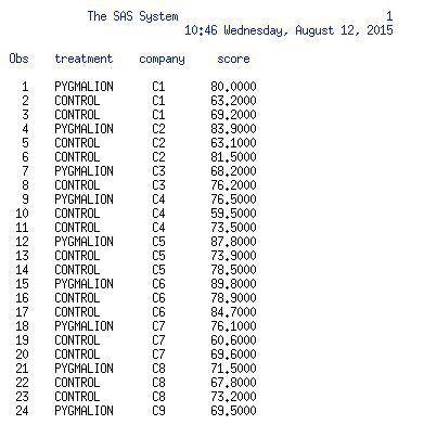
The data is following below.

Reference : Ramsey and Schafer (1997) The Statistical Sleuth, Duxbury Press, p. 365. The Pygmalion effect.


1. Two Way ANOVA with Interaction (Interaction Model & Hypothesis)  
The model with interaction :
$Y_{i}=\beta_{0}+ \beta_{1}I_{pyg,i}+ \beta_{2}I_{comp1,i}+...+\beta_{10}I_{comp9,i}$
                                        $+\beta_{11}I_{pyg,i}\cdot I_{comp1,i}+...+\beta_{19}I_{pyg,i}\cdot I_{comp9,i}+e_{i}$

$H_{0}:\beta_{11}=\beta_{12}=...=\beta_{19}=0$ (all possible interactions)
$H_{1}$ : at least $\beta_{1i}$ is not equal to 0

1.1 SAS Code and Result
 
We can create the Two-Way ANOVA by using proc glm. There are two factors; company and treatment. And we are also interested in interaction terms so that out model should be score=company | treatment, which | creates interactions. The another way to create interaction term is score=company treatment company*treatment.  
 

After running the SAS code above, the overall ANOVA results are following below.

In the interaction (company*treatment), the F value is 0.67 with high P-value (0.7221).
As we get a high P-value, we fail to reject the null hypothesis which means all possible interaction terms can be considered to 0. Therefore, our next model is an additive model which excludes the interaction terms.


2. Two Way ANOVA w/o Interaction. (Additive Model & Hypothesis)
The model w/o interaction:
$Y_{i}=\beta_{0}+ \beta_{1}I_{pyg,i}+ \beta_{2}I_{comp1,i}+...+\beta_{10}I_{comp9,i}$

2.1 The First Question - SAS Result and Conclusion 
Our first question is there is a difference in mean score between Pygmalion and the control groups!!
$H_{0}:\beta_{1}=0$ 
$H_{1} : \beta_{1}$ is not equal to 0

As our interest is to find a difference between Pygmalion and the control groups, so we need to look at the treatment source. As we have a small P-value (0.0119), so we reject the null hypothesis which means there is a evidence of a difference in mean score between them.
Note that F value is distributed by F(# beta being tested, # degrees of freedom of SSE) = F(1,18)

However, in the diagnostics for score matrix, we can see a decreasing variance estimate pattern. Even though we have a small P-value, the evidence of our conclusion is week.

2.2 The Second Question - SAS Result and Conclusion
Our second question is there are differences in companies!!
$H_{0}:\beta_{2}=\beta_{3}=...=\beta_{10}=0$ 
$H_{1}$ : at least one $\beta_{2}...\beta_{10}$ is not equal to 0
 

As our interest is to find a difference among 10 companies, so we need to look at the company source. As we have a high P-value (0.1484), we fail to reject the null hypothesis which means there is no evidence of difference among companies. 
Note that F(9,18) = F(# beta's being tested which are beta 2~10, # d/f of SSE)

Combining two question conclusion, our final model will be $Y_{i}=\beta_{0}+\beta_{1}I_{pyg,i}$


3. Model Checking
In the diagnostic panel, we can see whether our assumptions are satisfied or not.
There is no outliers, and normality looks ok. However, we have a concern of decreasing variance. Another assumption is independent observation which we assume that platoons were picked at random and were not interacting. 

Case Study: The Spock Conspiracy Trial, in SAS (by using proc glm)

Case Study: The Spock Conspiracy Trial in SAS
The main question is there is evidence that women underrepresented on Spock judges venire when compared to other judges?

1. SAS Code
Please refer to the previous post how to read the data file by using infile code, and sort into two groups; 'SPOCKS' and 'OTHER' by using if statement. This SAS code demonstrates how to use proc glm for comparing two groups. The class statement in proc glm makes dummy variables. In order to print the estimates of the beta's, then we need to put the solution statement.

2. SAS Code - Output List

If you run the SAS code above, you can see the result list below. From the class statement, we can see there are two levels, Poscks and Other. And we need to focus on Type III model ANOVA and Solution.   

 

3-(1). SAS Result -  Class Levels

As you can see the result below, there are two levels created, Other and Spocks.

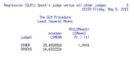
3-(2). SAS Result -  Least Squares Means

In this SAS output, we can see the least squares means for each level. Our hypothesis is that the LSMeans of the level Spock is equal to the LSMeans of the level Other.

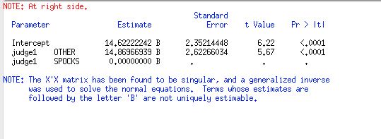
3-(3). SAS Result - glm solution   

From the solution statement, we can get the estimates of the each beta's. And each parameter has small p-values (less than 0.0001), so parameters are significant.
The equation will be pcwomen = 14.622 + 14.870*Other

3-(4). SAS Result - Type III model ANOVA    
F-value will be given in the Type III model ANOVA output. From the previous post regarding the two sample t-test in SAS, the pooled t-value was 5.67. Note that the squared pooled t-value is equal to the observed F value, which is 5.67*5.67=32.15.

4. Overall conclusion    
In order to compare the means of the two groups, we can use two sample t-test, SLR with 1 dummy variable or one-way ANOVA with two groups by using different statements. Of course each method has the same conclusion!!

Case Study: Two Sample T-Test in SAS

 

Case Study: The Spock Conspiracy Trial in SAS
The main question is there is evidence that women underrepresented on Spock judges venire when compared to other judges?


1. SAS Code
Read the data file by using infile code, and sort into two groups; 'SPOCKS' and 'OTHER' by using if statement. For the box plot, use the proc sgplot, and for the t-test use the porc ttest code.

 

2. SAS Code - Output List

If you run the SAS code above, you can see the result list below. There are two results; Sgplot (box plot) and T-test.

3. SAS Result - Box plot 

If you click the the SGplot Procedure, then you can see the boxplot output. This plot will be stored in PNG file as we put the ods graphics on statement.

 

Are the mean of two groups significantly different? Also, in 'OTHER' group, there might be suspected outlier. We should keep in mind about it and see the t-test result.

4. SAS Result - T-test & Conclusion

We are going to check those two results; T-test and Q-Q plots.

 

In the t-test, we see the Satterthwaite method as the variance of two groups are unequal. So, the t-value is 7.16 which p-value is less than 0.0001. Therefore, as we have a small p-value, we can conclude that we reject the null hypothesis. (The null hypothesis is that the mean of two groups are equal)  
 

In order to assess assumption of normality of the residuals, we should see the Q-Q plot (quantile quantile plot). From the Q-Q plot, it appears to be normally distributed, as most circles are close enough to the line.  

Case Study: SLR with 1 dummy variable in R

 

Case Study: The Spock Conspiracy Trial in R
The main question is there is evidence that women underrepresented on Spock judges venire when compared to other judges?

 

1. Prepare Data

If you don't have the data set, just follow procedure below; install a package and load the package. Our case study data set is called "case0502".

 

2. Make a Boxplot
Our goal is to compare the mean values between Spock's and other judges (1~6). First of all, we can make a bloxplot displaying the 5 statistics: minimum, first quartile, median, third quartile, and maximum.  

 

3. Conduct the SLR 

First, we divide into two groups: Spocks' and others by using ifelse function as we want to compare means of two groups. And then conduct the simple linear regression by using lm function. The response variable is the "percent" and the explanatory variable is a "twogroup" which is a dummy variable.  

 

4. Conclusion  

If we use anova( ), then we can see the one-way ANOVA table above. The main idea is that between groups SS (twogroups Sum sq=1600.6) is larger than withing groups SS (residuals sum sq=49.79), there is evidence that means are different. Therefore, as we have a small p-value (1.03e-06), there is strong evidence in mean difference between two groups.  
Remark) We will get the same conclusion if we conduct the SLR. More information, Click! 

 

- Reference: http://www.inside-r.org/node/159733  

 

 

Case Study: t-test in R

Case Study: The Spock Conspiracy Trial in R
The main question is there is evidence that women underrepresented on Spock judges venire when compared to other judges?


1. Prepare Data  
If you don't have the data set, just follow procedure below; install a package and load the package. Our case study data set is called "case0502".

2. Make a Boxplot
Our goal is to compare the mean values between Spock's and other judges (1~6). First of all, we can make a bloxplot displaying the 5 statistics: minimum, first quartile, median, third quartile, and maximum.  

 

3. Conduct the t-test

The data consists of 7 subgroups: A, B, C, D, E, F, and Spock's. We want to compare the mean of Spocks vs. other judges, so firstly we make two subgroups. And then conduct the two sampe t-test by using t.test.  

 

The variance of each group is not the same, so we use the Satterthwaite approximation. The degrees of freedom is calculated by Satterthwaite approx. formular.  

4. Conclusion

The null hypothesis is that there is no difference in mean between Spock's and other judges. As we have a small p-value (1.303e-06), we reject the null hypothesis so that there is strong evidence in difference between two groups.

Remark) We will get the same conclusion if we conduct the SLR. More information, Click!



- Reference: http://www.inside-r.org/node/159733 

Two Sample T-test for Comparing Two Means

1.Two Sample T-test for Comparing Two Means  
When do we use?
- Suppose we have two random samples which are from population 1(X) and population 2 (Y),
our interest is to compare those two population means. In this case, small sample size will be fine. (When we have large enough sample size, then we use Z-test.)  

Assumption?
- The two samples are identically independently distributed(iid) from approximately Normal populations. And Two samples are independent of each other. 

Hypothesis?
- There is no difference between two population means. $H_{o}=\bar{X}-\bar{Y}=D_{0}=0$

Test statistics?
- $t_{obs}= \frac{(\bar{X}-\bar{Y})-D_{0}}{se(\bar{X}-\bar{Y})}$ Wait!! How do we estimate the standard error of mean difference?


1.1. Pooled Two Sample T-test
When the population variances can be assumed to be equal, we use pooled two sample t-test!
Pooled variance estimate : $S_{p}^2= \frac{ (n_{x}-1)S_{x}^2 + (n_{y}-1)S_{y}^2 }{ n_{x}+n_{y}-2}$

Test statistics?
- $t_{obs}= \frac{(\bar{X}-\bar{Y})-D_{0}}{\sqrt{S_{p}^2( \frac{1}{n_{x}} +\frac{1}{n_{y}})}} \sim t_{n_{x}+n_{y}-2}$, Under the null hypothesis.


1.2. Two Sample T-test using Satterthwaite Approximation  
When the population variances cannot be assumed to be equal, we use Satterthwaite approximation.

Test statistics?
- $t_{obs}= \frac{(\bar{X}-\bar{Y})-D_{0}}{ \sqrt{ \frac{S_{x}^2}{n_{x}}+ \frac{S_{y}^2}{n_{y}}}} \sim t_{\gamma}$, Under the null hypothesis, where  $\gamma = \frac{ (\frac{S_{x}^2}{n_{x}} + \frac{S_{y}^2}{n_{y}})^2}{\frac{(\frac{S_{x}^2}{n_{x}})^2}{n_{x}-1} + \frac{ (\frac{S_{y}^2}{n_{y}})^2}{n_{y}-1} }$ d/f.
Here, this degrees of freedom is calculated by Satterthwaite approximation which rounds down to the nearest integer. 



2. Case Study: The Spock Conspiracy Trial
Description

In 1968, Dr. Benjamin Spock was tried in Boston on charges of conspiring to violate the Selective Service Act by encouraging young men to resist being drafted into military service for Vietnam. The defence in the case challenged the method of jury selection claiming that women were underrepresented. Boston juries are selected in three stages. First 300 names are selected at random from the City Directory, then a venire of 30 or more jurors is selected from the initial list of 300 and finally, an actual jury is selected from the venire in a nonrandom process allowing each side to exclude certain jurors. There was one woman on the venire and no women on the final list. The defence argued that the judge in the trial had a history of venires in which women were systematically underrepresented and compared the judge's recent venires with the venires of six other Boston area district judges.

 

Reference: http://www.inside-r.org/node/159733 

The main question is there is evidence that women underrepresented on Spock judges venire when compared to other judges?

*Two sample t-test in R 
If you are not ready...
> install.packages( "Sleuth3" )
> library(Sleuth3)
> attach(case0502)
For more information> Click!! :D

* SLR in R 
For more information> Click!! :D

* Two Sample t-test in SAS
For more information> Click!! :D